Bidirectional Decoding: <br> Robots Should Plan Long and Adapt

The past year has seen a tremendous increase in efforts to scale up robotic data collection with projects like Open X-Embodiment, Droid, BridgeData, UMI, etc. Such large datasets of expert demonstrations, coupled with strong behavior cloning algorithms, can help robots learn complex skills, from folding shirts to cooking shrimp. These datasets generally encompass a diversity of strategies for every task aimed towards teaching a diversity of skills. They contain demonstrations from a variety of experts with different preferences and proficiency levels—for example, demonstrations from left-handed experts versus right-handed ones, demonstrators that are more adept at a task than others. They also contain various temporal dependencies within each trajectory—for example, a trajectory can consist of various subtasks that are being completed one after the other. These become latent variables underlying trajectories (e.g. the skill-level of the demonstrator carrying out the trajectory) or parts of trajectories (e.g. the subgoal that the subsection of the trajectory is aiming to achieve) in the data.

Learning policies from such datasets is one aspect of the problem but not the only one. Recent generative behavioral cloning policies like diffusion policies can capture multiple behavior modes. However, optimally executing a strategy is another aspect of the problem altogether. The natural framework in which we can analyse this is test-time decoding from these policies.

Having learnt a diversity of strategies, one of the challenges is in choosing the right strategy. For example, we would want the robot to correctly react to unexpected changes in the environment. We would also want the robot to prefer the more optimal strategies it has learned and execute them instead of having an almost uniform distribution over all strategies. The optimal strategy could be characterized in many ways - for example, it could be the most "efficient" way to complete the task or it could be the solution that reacts in the best manner to the environment. This is non-trivial given how optimal a strategy is an unlabelled latent and requires both powerful learning algorithms and inference mechanisms.

Another challenge is in consistent execution of a given strategy. In other words, once a strategy has been sampled at a time step, the robot needs to commit to that strategy and execute in a coherent manner; it must not hop from one strategy to another like switching from being left-handed to right-handed while picking up a glass of water. This requires learning temporal dependencies, identifying latent variables hiding in the demonstrated trajectories and sampling actions in a manner that the latent variables remain consistent.

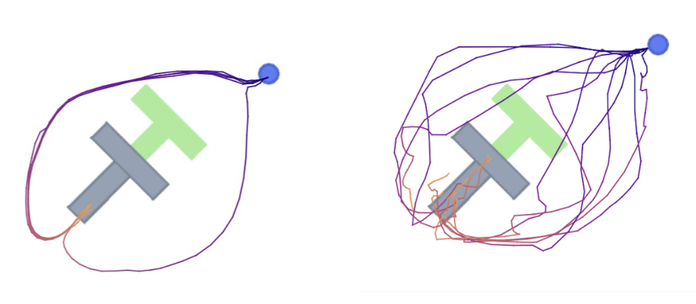
Here is an illustration—-consider the Push-T task where the agent (the blue circle) needs to push the grey T-shaped block to cover the green-colored target. There are multiple routes that the agent can take to get to the tail of the block and start pushing it. We want an agent to be able to take any one of these two routes consistently, like the one in the left figure. But the right figure shows an agent that fails to commit - it often starts taking one route and then switches to the other, leading to jittery trajectories.

Therefore, we have a two-pronged challenge. Firstly, we need our robot to choose the more optimal strategies during sampling. Secondly, we need the robot to consistently execute whichever strategy it selected.

One possible way to at least partially solve this could be to use very long contexts. Conditioned on long contexts, the policy, in theory, should be sampling from the same strategy in a temporally coherent manner. However, in practice, large context lengths end up hurting performance as models often learn spurious correlations. We illustrate this in the Push-T task with diffusion policies. This is also the reason why most state-of-the-art robotic foundation models like OpenVLA and $\pi_0$ use very short context lengths (often lengths of size 1). We will return to this discussion on context length later.

This is not a novel goal by any means. In fact, over the past year, researchers have discovered interesting techniques to achieve some of these goals. One interesting practice has been something called "action chunking" used by most state-of-the-art methods like $\pi_0$. Under this paradigm, at a state, our agent does not only generate the next action. Instead, it models the join distribution of the next $ p $ actions: $$\pi(a_{t}, a_{t+1}, \ldots, a_{t+p} | s_{t}, s_{t-1},\ldots,s_{t-c}).$$

Here, $p$ is referred to as the prediction horizon and $c$ is the context length. Having modelled this joint probability of the next $p$ actions, the agent executes the next $h$ (where $h$ is between 1 and $p$) actions straight-away without replanning at each timestep. We call $h$ the action horizon. We call this an "open-loop operation"--since we do not get feedback from state observation and, instead, "blindly" execute the $h$ actions. In contrast, "closed-loop operations" refers to sampling processes where the agent observes every state at every timestep and plans all over again.

The effects of action chunking are not well-understood. While some works like Diffusion Policies and ACT have found them to be critical, others have found them to be counterproductive at times, like Behavior Transformers (BeT) and Vector-quantized Behavior Transformers (VQ-BeT). Even for a given method, they tend to sometimes be useful and sometimes counterproductive-for example, VQ-BeT found it to be harmful for every task other than Push-T. Some papers have hypothesized that action chunking increases temporal coherence although this is not really made rigorous. The alternative hypothesis is that action chunking increases smoothness of trajectories. However, these arguments do not always hold and are more often than not dependent on the environment that the agent is operating in and the nature of the task. In fact, there have been public calls for a stronger analysis of the strengths and weaknesses of action chunking.

Our first goal in our paper is to understand the strengths and weaknesses of action chunking. We will compare the performance of a policy with shorter action horizon and the performance of one with a larger action horizon. Suppose an agent executes action chunks of length $h$ and suppose this action chunk is generated conditioned on the observations of the last $c$ states. Then, we will refer to this agent as a $(c,h)$-model. In contrast, the expert demonstrator clearly only executes one action at a time, so their action chunk is of length 1 but the action is assumed to be dependent on, at most, the last $k$ observations. We would like to compare between a $(c, h)$-model and a $(c, h+d)$-model (i.e., an agent with larger action chunks) -- in particular, we want to determine which model can imitate the expert distribution better. Here is an illustration for when these two policies' action chunks are aligned:

Note that the larger action chunk model cannot observe more of the recent states which the smaller action chunk model can. On the other hand, the larger action chunk model can condition on some more past states that precede all the context that the shorter action chunk model can condition on. Our analysis starts off with asking the following question: how important is a state that a policy has observed and how important is a state that was not observed?

In the paper, we provide a rigorous mathematical formulation of these terms. We formulate the expected advantage from observing some states by, roughly, comparing the performance of two policies - one that observes the states and one that does not, with all else equal between the two policies. More formally, consider a policy that has observed (i.e. can condition on) a state $s_t$ denoted by $\pi(s_t)$ and a policy that does not condition on $s_t$ (but conditions on all other information that $\pi(s_t)$ can observe) denoted by $\pi$. Then, $$\alpha_{\{s_t\}} = \min_{\pi} \mathbb{E}_G\left[\mathcal{L}(\pi, \pi^*) \mid C \right] - \min_{\pi(s_t)} \mathbb{E}_G\left[\mathcal{L}(\pi(s_t), \pi^*) \mid C \right]$$ where $\mathcal{L}$ is a non-linear convex function measuring the prediction error with respect to demonstrations, $C$ is the set of all variables that both policies can condition and $G$ is the set of all remaining variables that the expert conditions on. One can easily prove, as we did in the paper, that context is valuable and therefore, $\alpha_{\{s_t\}} \geq 0 $.
On the other hand, we formulate the maximum disadvantage from not observing some states as the maximum divergence attained by a policy that, roughly, infers all of these unobserved states incorrectly. More formally, consider a policy that has not observed (i.e. cannot condition on) a state $s_t$ denoted by $\pi$. After inferring the state to be $\hat{s}_t$, we write this policy as $ \pi(\hat{s}_t)$. Then, $$\mathcal{L}(\pi(\hat{s}_{t} \neq s_{t}), \pi^*) \leq \epsilon_{\{s_t\}}.$$
We will denote the advantage that $\pi_h$ gains from the observed recent states by $\alpha_f$ and the inference disadvantage it incurs from the earlier unobserved states by $\epsilon_b$, whereas $\pi_{h+d}$ conversely gains $\alpha_b$ but incurs $\epsilon_f$. In the paper, we proved the following which intuition suggests should hold true:

Importance is one half of the story. An unobserved state might be extremely important but we need not incur the full penalty of not observing it if there is a high likelihood that the model can infer having visited that state. As such, we also care about the probability of inferring that a state was visited. This is heavily tied to the stochasticity of the environment (see Appendix C.2): let $P_f := P(S_{t}=g_t|S_{t-1}=g_{t-1},a_{t-1})$ where $g_t$ and $g_{t-1}$ are the ground truth states in the deterministic environment. In deterministic environments, $P_f = 1$, whereas in stochastic settings, $P_f$ is smaller. On the other hand, let $P_b := P(S_{t}=g_t|S_{t+1}=g_{t+1})$. Since $P_b$ is not conditioned on any action, it has higher entropy in general. In stochastic environments, $P_b$ is small. Note: we glossed over some details needed to define $P_f$ and $P_b$ more formally but the core idea remains the same.

The fact that a policy has to infer missing information is not really much of an additional assumption we are making. For instance, we can always write $$ \pi_{(c, h)}(a_t|s_{t-h-c:t-h},a_{t-h:t-1}) = \mathbb{E}_{s_{t-k:t-h-c-1},s_{t-h+1:t} \sim \hat{P}}\left[\pi_{(k, 1)}(a_t|s_{t-k:t})|s_{t-h-c:t-h}, a_{t-h:t-1}\right].$$ However, here, $ \hat{P} $ could differ from one learner to another. To simplify this problem, we assume that an optimal learner can capture the true environment dynamics allowing us to say $ \hat{P} = P $. In other words, with sufficient data (since we are talking about the optimal learner), the learner can infer the missing states' distribution correctly.

This allows our theoretical analysis to ignore all other details and abstract the problem to the following: how much advantage does a policy gain from observing some states and how much disadvantage does it incur from not observing some states? Both of these questions are heavily tied to (1) the length of temporal dependencies (2) the change in the strength of temporal dependencies over time steps and (3) the stochasticity in the environment.

We can bound the difference in divergence attained by the following proposition:

Proposition 1 (Consistency-Reactivity Inequalities): Let $\mathcal{L}$ be a non-linear convex function measuring the prediction error with respect to demonstrations. Let $\mathcal{S}^+ \subset \{s_{t-k:t}\}$ be the states both the $(c, h)$ and the $(c, h+d)$ policies observe and let $\mathcal{S}^- := \{s_{t-k:t}\}\setminus\mathcal{S}^+$. Similarly, let $\mathcal{P}^+ := \{a_{t-h:t-1}\}$ and $\mathcal{P}^- := \{a_{t-h-d:t-h-1}\}$. Let $C := \mathcal{P}^+ \cup \mathcal{S}^+$, $G := \{a_t, z_{t-k:t}\} \cup \mathcal{P}^- \cup \mathcal{S}^-$. Then, we can bound the expected loss of the $(c, h+d)$-policy and the $(c, h)$-policy as: $$\alpha_{f} - \epsilon_{b}(1 - P_b^{2d}) \leq \min_{\pi_{h+d}} \mathbb{E}_{G} \left[\mathcal{L}(\pi_{h+d}, \pi^*) | C \right] - \min_{\pi_{h}} \mathbb{E}_{G} \left[\mathcal{L}(\pi_{h}, \pi^*) | C \right] \leq - \alpha_{b} + \epsilon_{f}(1 - P_f^{2d})$$

Intuitively, the advantage of each policy stems from the additional information it has access to ($\alpha_{f}$ for $\pi_h$ and $\alpha_{b}$ for $\pi_{h+d}$) while the disadvantage is bounded by the maximum divergence arising from inferring missing information incorrectly ($\epsilon_{b}(1 - P_b^{2d})$ for $\pi_{h}$ and $\epsilon_{f}(1 - P_f^{2d})$ for $\pi_{h+d}$).

In near-deterministic environments, inferring the unobserved, recent states is easy for the larger chunk (see figure 2 above) because it has access to the actions taken during these time steps. Therefore, the larger chunk model has strictly more information as it also remembers the distant past states that the shorter action chunk has forgotten. When the action to be taken is temporally dependent over long context, a larger action horizon is going to perform better. This is shown in the following result:

Corollary 2: In a highly deterministic environment, if $a_t$ is temporally dependent on at least one state in $\{s_{t-h-c-d:t-h-c-1}\}$ and $\epsilon_{f}$ is finite, then $$\min_{\pi_{h+d}} \mathbb{E}_{G} \left[ \mathcal{L}(\pi_{h+d}, \pi^*)| C \right] < \min_{\pi_{h}} \mathbb{E}_{G} \left[\mathcal{L}(\pi_{h}, \pi^*)| C \right]$$

Conversely, in highly stochastic environments, inferring the unobserved states is challenging, regardless of whether the actions are known. However, the recent states are likely more important than earlier states for predicting the current action since the strength of temporal dependencies, quite likely, decrease over time steps. In this case, the longer action chunk will perform worse:

Corollary 3: In a highly stochastic environment, if temporal dependency decreases over time, i.e., $\alpha_f > \epsilon_b$, then $$\min_{\pi_{h+d}} \mathbb{E}_{G} \left[\mathcal{L}(\pi_{h+d}, \pi^*)| C \right] > \min_{\pi_{h}} \mathbb{E}_{G} \left[\mathcal{L}(\pi_{h}, \pi^*)| C \right]$$

We glossed over several details on our set-up but, hopefully, the core point remains clear. There is no universally optimal action horizon across all conditions. Determining the appropriate action horizon requires careful consideration of (i) the length of temporal dependencies in the demonstrations, how they decrease over time steps, and (ii) the level of transition stochasticity present in an environment. When both temporal dependencies and environmental stochasticities are significant, the vanilla action chunking approach leads to an inherent trade-off between these two competing factors.

One way forward from here could be to always select the length of action chunks on the basis of how stochastic the environment is and the length of temporal dependencies in demonstrations. However, both of these are largely intractable. One could choose action chunking in dynamic environments only but it’s certainly possible that in many of the timesteps, there is no noise in which case we would want the temporal consistency action chunking brings whereas in other timesteps, where we encounter noise, we would want higher reactivity.

We validate this analysis through a diagnostic simulation. The environment we consider is a 2-dimensional grid world where $x \in [-10, 10]$ and $ y \in [0, 10]$.

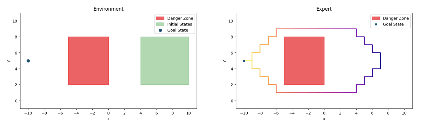
The initial state is randomized and the goal of any agent is to reach the goal state by avoiding the danger zone. The environment can be stochastic which is characterized by a noise level $\delta$. So, for any action, with probability $ 1 - \delta$, the action is successfully executed and with probability $\delta$, the agent just stays idle. The expert policy has a few characteristics. From any initial state, with equal probability, the expert chooses to get to the goal state by first going upwards or by going downwards. Once this strategy is selected, the expert commits; they will never go upwards and then start going downwards again. Notice that our characterization of stochasticity is also such that even if the environment is stochastic, the expert will not go in the opposite direction to the one they intended to go. The other characteristic is that the expert carries out a staircase-like trajectory unless it's at the borders of the state space i.e., no two consecutive actions will be the exact same. These characteristics introduce both global and local latents underlying the expert trajectories and we will remember them as we analyse how temporally consistent each policy is.

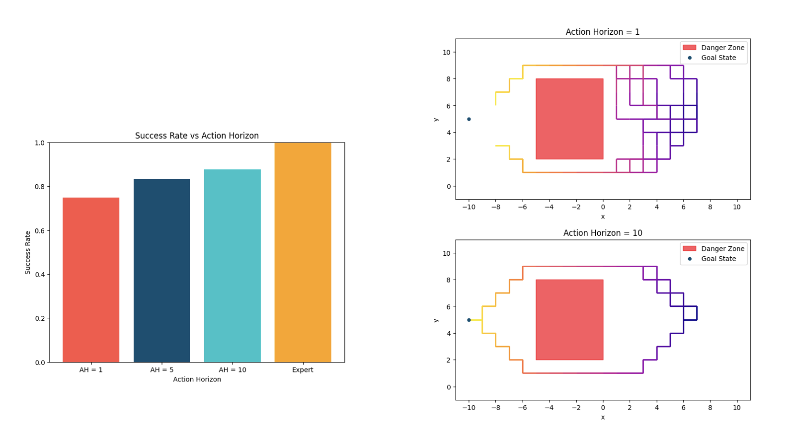
In the static environment, we notice that increasing the action horizon yields better performance. The reason for this is that shorter action horizon does not capture the temporal dependencies across actions - with closed-loop operations, the policy often ends up not being able to execute the staircase-like motion that the expert does and often chooses less time-efficient trajectories causing it to not reach the goal state in time. In contrast, the long horizon policy imitates the expert near perfectly.

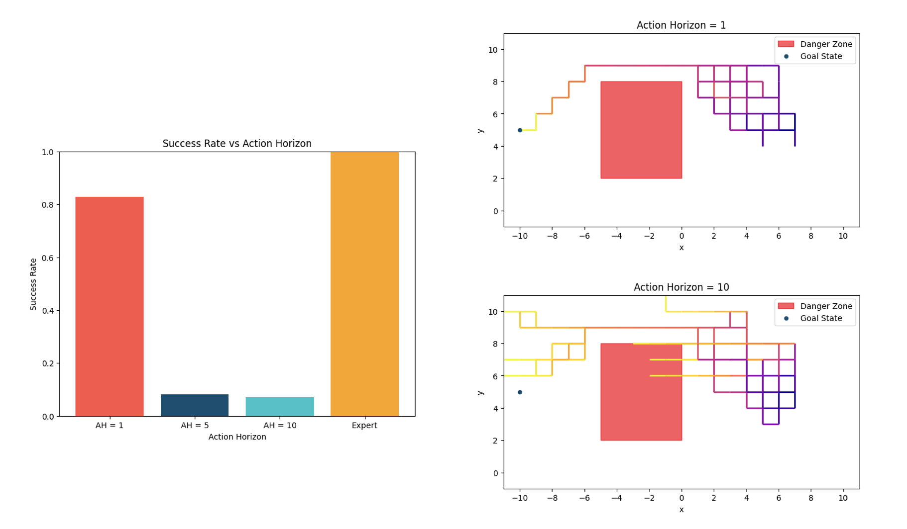
In the highly dynamic environment, we notice that increasing the action horizon yields worse performance. The long horizon policy fails to react to the environmental stochasticity causing it to infer states incorrectly and hit the danger zone or leave the state space altogether. Even though the short horizon policy cannot perfectly capture the temporal consistencies, it reacts to stochasticity better causing it to be able to reach the goal state more often. We further validated our theory in more standard imitation learning settings too which we shall touch upon when we discuss the results.

Our approach to solving this problem was to think about increasing temporal consistency within closed-loop action chunking. In other words, we maximize reactivity by using closed-loop operations and then increase temporal consistency through resampling methods. Apart from the fact that this increases reactivity, there is a robustness argument too -- an open-loop policy has to get good at inferring unobserved states which is both challenging and subject to generalization difficulties whereas a closed-loop policy can always observe the states.

The first step is to think about being consistent with a strategy we selected in a previous timestep. One simple yet effective way to do this is to use backward coherence: suppose we are at time $t$ and we want to sample action $a_t$. One way to do this is to first sample an action chunk $(a_{t},\cdots,a_{t+p})$ that is "coherent" with action chunks taken previously and then only take the first action $a_t $ in the chunk. We sample $n$ action chunks at timestep $t$ and then select the one that minimizes a loss that quantifies how incoherent the chunk is with previous steps. Once we have done so, we only take the first action in the chosen chunk. More formally, we use the action chunk selected at the previous time, ${a}^{(t-1)}_{t-1}, \cdots, {a}^{(t-1)}_{t+p-1}$, and select the action chunk that minimizes the weighted sum of Euclidean distances across the $p-1$ overlapping steps: $$\mathcal{L}_B(a^{(t)}) = \sum_{\tau=0}^{p-1} \rho^\tau \left\| a^{(t)}_{t+\tau} - {a}^{(t-1)}_{t+\tau} \right\|_2.$$ We found other approaches like exponential moving average (EMA) to be fairly powerful as well. However, the issue with simply averaging is that the resulting action could end up being one that is very low probability in our policy distribution. Our method, instead, takes an "$\arg\min$" over actions we sampled from the policy so we only take an action that the policy does choose and is consistent. Empirically, we observed that averaging leads to loss of precision

The backward coherence incentivizes our policy to take actions that are consistent with previous actions. However, consistency is only one part of the problem. Consistently executing suboptimal trajectories would continue to be a problem. We would want our robot to, generally, select more optimal strategies and then stick to it. The notion of "optimal strategies" is subjective. One aspect of it is the observation that expert demonstrators tend to make long-term plans and so, we would want our robot to select more long-term strategies too. We wouldn't want it to select a trajectory to pick up the jug of water only to find out after 10 steps that there is an obstruction on this trajectory - it should plan ahead to avoid that obstruction in the first place.

One naive approach for this could be to just train policies that are exceptionally long-horizon. However, that is also exceptionally data and compute-expensive. A simple, yet effective approach to do this is to use contrastive sampling, fairly similar to contrastive decoding in NLP. We introduce a forward contrast objective to identify and reject these suboptimal plans. At the core of the forward contrast is to compare each candidate plan with two sets of reference samples: one set from a stronger policy and the other set from a weaker one. We use a well-trained model built with a long prediction horizon as the stronger policy, and a model with a shorter prediction horizon or from an early underfitting checkpoint as the weaker policy. Intuitively, either choice of the weaker policy cannot capture long-term planning as effectively as the stronger one. Our forward contrast loss is thus framed as minimizing the average distance between a candidate plan and a set of positive samples while maximizing its average distance from the negative ones.

$$\mathcal{L}_F = \sum_{a^{+} \in \mathcal{A}^{+}} \sum_{\tau=0}^{p'} \left\| a^{(t)}_{t+\tau} - a^{+}_{t+\tau} \right\|_2 - \sum_{a^{-} \in \mathcal{A}^{-}} \sum_{\tau=0}^{p'} \left\| a^{(t)}_{t+\tau} - a^{-}_{t+\tau} \right\|_2,$$ where $\mathcal{A}^{+} = \mathcal{A} \setminus \{a\}$ is the positive set predicted by the strong policy $\pi$, $\mathcal{A}^{-}$ is the negative set predicted by the weaker one $\pi'$, and $p'$ denotes the shortest prediction horizon between the two policies.

Putting it all together, we have our final sampling algorithm. Suppose, we have a generative policy with context length $c$ and prediction horizon $p$ and an action chunk sampled at time $t$: $$a \sim \pi_\theta(a_{t}, a_{t+1}, \cdots, a_{t+p} | s_{t-c}, s_{t-c+1},\cdots,s_t).$$ We cast the problem of closed-loop action chunking as searching for the optimal action among a batch of plans sampled at each time step, $$a^* = \arg\min_{a \in \mathcal{A}} \mathcal{L}_B(a) + \mathcal{L}_F(a),$$ where $\mathcal{A}$ is the set of sampled action chunks, $\mathcal{L}_B$ and $\mathcal{L}_F$ are the two criteria.

This final form of our sampling method allows us to see another reason why both the criteria are important. Suppose, we used only backward coherence. If we sample a sufficiently large number of action chunks, it is possible that we may sample a chunk that is very close to the previous timestep's chunk but has low probability, because it is not sufficiently reactive to the current observation. As such, even though it is coherent, executing this chunk is not optimal. Forward contrast corrects for this by ensuring that the sampled chunk is not only coherent but also close to the optimal chunk in the sense that its probability of being sampled by the optimal policy is high. While the base algorithm just takes the argmin over both criteria, one can use more clever techniques from constrained optimization (like double descent) for a better balance of both criteria.

We go over some of the experiments that we conducted to test BID. We want to (1) validate our theory i.e., test whether closed-loop operations are truly better in stochastic environments (2) test whether BID outperforms other action decoding methods in both static and noisy environments.

Simulation Experiments

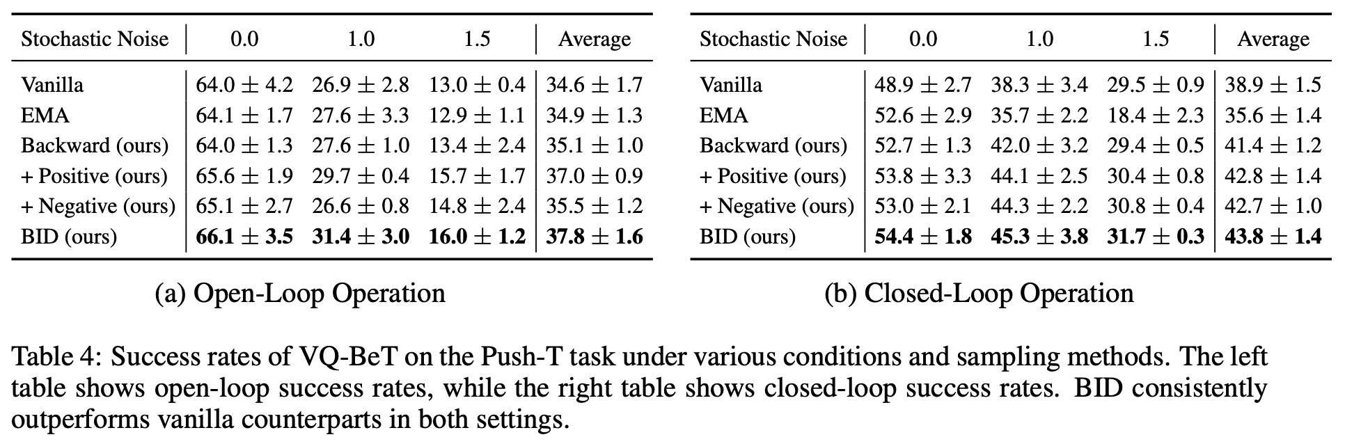
We first test BID on Vector-Quantized Behavior Transformers in the Push-T task. The results are summarized below. We observe that in the static setting, open-loop operations tend to be better than closed-loop operations, as suggested by Corollary 2. BID still outperforms Vanilla open-loop. However, in the noisier settings, closed-loop operations always seem to be the best choice wherein BID gains a significant performance boost compared to the vanilla alternatives, as suggested by Corollary 3. BID achieves significant improvement compared to other closed-loop operations even in static settings.

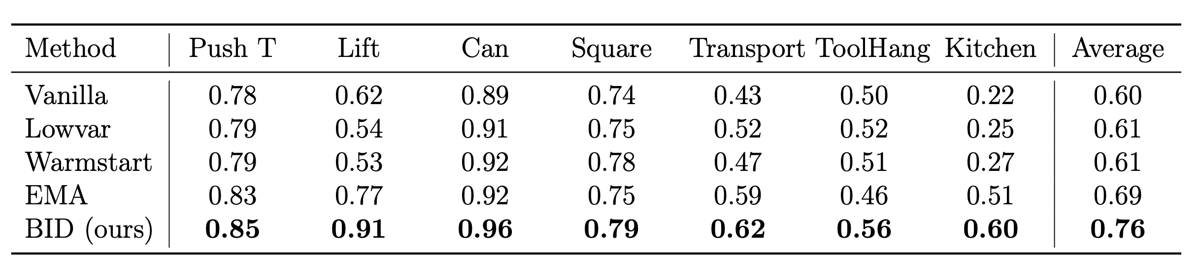
We also tested BID on Diffusion Policies and compared against 4 baseline methods and found that BID is significantly more robust.

Real World Experiments

We tested BID on two real-world experiments in dynamic environments. For both, we deployed BID on top of a pre-trained diffusion policy.

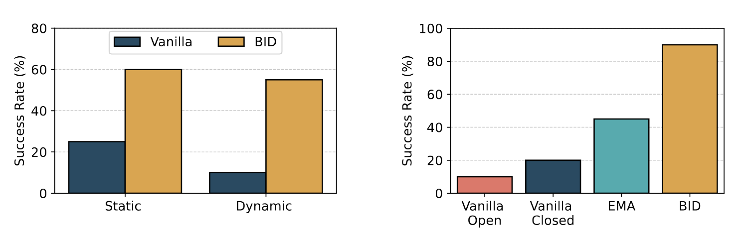
For the first task, we consider a task where the robot is to deliver an object held in its gripper into a cup held by a human. To introduce stochasticity, the cup is moved while the robot completes the task. For both the static and the dynamic settings, we see that BID gains almost 2x the success rate compared to vanilla closed-loop operations, as shown below. For the second experiment, we consider a cup rearrangement task. The robot must pick up a cup that is moved while it is completing the task. After that, the robot must place the cup on a nearby saucer. We use the public checkpoint from UMI , without any further fine-tuning, and compare BID with vanilla (both open and closed-loop) and EMA. The results are summarized below. We observed that open-loop operations degrade very significantly in dynamic settings where BID outperforms all other baselines by at least two times. In static settings, we observe that BID matches the peformance of baseline methods. Notably, the UMI dataset did not contain demonstrations in a stochastic environment and yet, BID performs well without further fine-tuning -- which reinforces our motivation that open-loop operations struggle with generalization due to the need to infer unobserved states.

I want to stress that the theoretical analysis relies on the assumption that the context length is small compared to the expert's memory horizon. In practice, context length in robotics is small. For example, diffusion policies use context length 2 whereas VQ-BeT use 5. Part of the reason for this is that, with insufficient data, long-context models often learn spurious correlations as opposed to the true temporal dependencies. I believe that as robotic data scales up, we can, more comfortably, extend context length and that would be beneficial. This extremely intuitive result has an extremely intuitive proof:

Proposition 4: Let $\mathcal{L}$ be a non-linear, convex function. Let $c < k$. Let $G := \{a_t, s_{t-k:t-c-1}, z_{t-k:t}\}$ and let $C := \{ s_{t-c:t}, a_{t-1}\}$. Then, $$\min_{\pi_{(c+1,h)} \in X_{+,+}} \mathbb{E}_{G} \left[ \mathcal{L}(\pi_{(c+1,h)}, \pi^*) \Big| C\right] \leq \min_{\pi_{(c,h)} \in X_{-,-}} \mathbb{E}_{G} \left[ \mathcal{L}( \pi_{(c,h)}, \pi^*) \Big| C \right].$$

However, I also believe that it is non-trivial to ask how much such data needs to scale up; real world robotic tasks are complex and it is possible that the scale of data needs to be significantly larger than that of, say, NLP. And even within NLP, whether context is truly being used properly or not is questionable. For example, it has been observed that language models tend to use information provided either in the beginning or the end of the context more than the information provided in the middle - to the extent that providing valuable information in the middle of the context might even be worse than not providing any information at all. The methods for conditioning on context are also an important area of research - a direction that I am personally excited about pursuing.

Eitherways, assuming we can learn from long contexts some time into the future, in that realm, it is possible that action chunking itself would not be necessary. The optimal learner, after all, is still a $(k, 1)$-policy. However, in that realm, contrastive sampling should still be a powerful method in improving the quality of strategies executed. Furthermore, our analysis assumed that all the important information is in the states visited in the past. It is important to question whether models need to also condition on past actions and what kind of consistency might come from that. Action chunking, afterall, does allow the model to condition actions on past actions within the chunk.